Journeying into XDP: XDPerimenting with DNS telemetry

By Luuk Hendriks
The XDP programs we’ve so far described in this series have been actively modifying DNS packets to perform functions such as response rate limiting (RRL), cookies and padding. This time, we’ll look into a passive BPF-program which enables us to plot graphs of DNS metrics without altering the DNS packets or touching the DNS software itself.
We'll discuss why we do this on the XDP-layer (as opposed to the on Traffic Control (TC) layer), and what design choices we make to get from raw packets to, eventually, a Prometheus+Grafana dashboard.
When, where and what to measure?
Our main aim for this work is to get insight into what a nameserver is doing. If we have to choose between collecting statistics on queries or statistics on answers, the latter will provide a better view of what the nameserver actually spends resources on. Consequently, as we are dealing with egress packets, we have to use the TC layer to deploy our BPF program.
However, that means we assess a packet that has gone through userspace already. Moreover, the nameserver could do all the statistics gathering and telemetry without the limitations we would face in doing the same in BPF/XDP. So instead, we will look at the queries coming in, and thus do our statistics gathering in XDP.
The benefit of assessing the queries instead of the answers provided by the nameserver software is we can now get insight into queries that might be dropped early on by that nameserver software. Perhaps because they are malformed, or because the query is for a totally different zone than the ones served by this nameserver. And because these queries will never be answered, the nameserver might not give any useful statistics on them. So focussing on incoming queries in XDP seems to provide more value than looking into outgoing answers at the TC layer.
Code-wise, there are a handful of differences between writing a BPF-TC program compared to XDP. Creation of maps, altering the packet headers and payload (which we do not need for this telemetry program) and tail calling are done in slightly different ways, but none of these are showstoppers. During this experiment, we actually tried this in both the TC and XDP layers, and both are perfectly feasible and viable ways of getting numbers on your DNS packets.
For our example, we will measure DNS queries, on the XDP layer. Using DNS-OARC's DSC for inspiration, we distill the main metric must be the query count and/or rate, parameterized by typical DNS information such as QTYPE and the QR-bit. Furthermore, we'd like to distinguish whether queries come in over IPv6 or IPv4, and gather some insights on the EDNS0 buffer sizes. In other words, we are dealing with many dimensions here.
Before we decide on how many parameters/dimensions we can handle, let's have a look at how we can actually keep track of such data in BPF.
Storing multi-dimensional data
We have plenty of BPF map types at our disposal, to keep track of anything in-between packets in BPF. But which of these fit our 'multi-dimensional' requirements?
We could use a bunch of simple MAP_TYPE_ARRAY-based counters for every possible parameter: A counter for A-record queries, a counter for AAAA-queries, a counter for queries coming in over IPv6, and so on. However, that way we immediately lose information on any possible correlations between these numbers. There is no way to say afterwards whether the A-record queries came in over IPv6 or IPv4, for example, or which EDNS0 size they carried.
Looking at man bpf, two of the available map types have a name that sounds promising for our use case:
MAP_TYPE_HASH_OF_MAPS
MAP_TYPE_ARRAY_OF_MAPS
Their names suggest they carry multi-dimensional data, and indeed they can. Unfortunately, it seems that these map types are limited to only one level of nesting, and, moreover, the 'parent' level has to be occupied at compile time. All in all, not the flexibility we had hoped for but to be fair, the intended use case for these map types is perhaps not what we are trying to squeeze out of them.
This is one of these cases where the solution turns out simpler than whatever direction we were thinking in. We can do this in a rather straightforward way by using nothing but a hashmap (MAP_TYPE_HASH). The implementation of the hashmap in BPF allows not only simple values to represent the key to be hashed, but also lets us define our own structs to be keyed on. Perhaps even more important, those keys themselves are actually stored in the map, so we can retrieve them later on.
Let’s compare this to writing P4 code, another programmable data plane paradigm: P4 offers constructs to hash one or more values (for example, DNS features as we do here) into an offset so we can read/write a value in a register at that offset. However, the values used as input for the hash function are not stored. Only if we process another packet with the exact same features going into the hashing function, we know what the value at the offset in the register represents, but only as long as we are processing that specific packet.
From a (higher level) application programming perspective this might not sound like a big deal (I always iterate over the keys of my hashmap, what's the fuss about?). However, keeping those keys around really makes certain tasks a lot easier in this data plane programming context.
Before we go into the actual C struct for keying our map, let's look at the consuming side of the metrics we will store in that map, and why we need to take this into account.
Cardinality
For this setup, we used the well-known combination of Prometheus and Grafana to ingest and store the metrics, and plot them, respectively. This means that the contents of our BPF hashmap needs to be output in a specific Prometheus format, which is human-readable and straightforward. For example, reporting that the number of queries for AAAA records (qtype=28) that came in over IPv4 (af=0) with the DO-bit set (do=1), is of value 1234, looks like:
queries_total{af=0, qtype=28, do=1} 1234Dissecting this line gives us the metric queries_total, parameterized by three features we can extract from the DNS query packet. Another line in the same output could represent the queries with the same DNS features but IPv6 (af=1) for transport:
queries_total{af=1, qtype=28, do=1} 2345Every combination of these parameter values results in a separate time series in Prometheus. Thus, every parameter adds a dimension of a certain size based on its different values. Storing the address family, for example, doubles the number of time series, as we expect two values (IPv4 and IPv6). In other words, the cardinality (the number of elements in the set) doubles.
For Prometheus, it is advised to not create metrics with a cardinality greater than 100k. Calculating the cardinality for our examples here, where |X| means 'the number of different values for X', shows we are still good:
|af| * |do-bit| * |qtype| =
  2  *     2    *   60    = 240
Note we used a rather large number for qtype. On many networks, the number of different qtypes might be far less, but let's be conservative with our estimations for now.
If we now also track EDNS0 sizes in, say, 20 buckets, and also track the AD-bit (0 or 1), and maybe track whether the incoming packets correctly have the query bit set (0 or 1), the cardinality increases to ~20k. Not quite yet the 100k limit (which is not a hard limit, only a recommendation) for Prometheus, but this shows how quickly things add up. On the BPF side though, we can represent most of these options in just a two or three-byte map key.
Clearly, this time it is not (only) BPF itself that is making us think twice about our design decisions in terms of resources and complexity.
The key is key
These are the features we use in our key, and the C struct they constitute:
| cardinality | |
|---|---|
| AddressFamily | 2 |
| qr-bit | 2 |
| do-bit | 2 |
| ad-bit | 2 |
| EDNS0 size buckets | 8 |
| qtype | 10 |
| tld | 75 |
| total cardinality | 96.000 |
Translated into the struct:
struct stats_key {
	uint8_t af:1;
	uint8_t qr_bit:1;
	uint8_t do_bit:1;
	uint8_t ad_bit:1;

	uint8_t no_edns:1;
	uint8_t edns_size_leq1231:1;
	uint8_t edns_size_1232:1;
	uint8_t edns_size_leq1399:1;
	uint8_t edns_size_1400:1;
	uint8_t edns_size_leq1499:1;
	uint8_t edns_size_1500:1;
	uint8_t edns_size_gt1500:1;

	uint8_t qtype;
	char tld[10];
};
This time, we calculated the cardinality based on different values we hoped are more representable for most networks (that is, in practice we expect 10 different qtypes to be more realistic than 60 different ones), but as always, your networks may vary.
Another take-away from this table is how we choose to do an aggregation step in BPF to reduce the cardinality by grouping EDNS0 sizes in bins. This reduces the cardinality of that single feature by three orders of magnitude.
Lastly, there is the top-level domain (TLD) feature. For operators hosting zones for multiple TLDs, being able to distinguish one from the other is useful when interpreting the numbers. In the table we listed the expected different values for the TLD to be 75, which might be an order of magnitude greater than most operators need. The number is chosen to max out the cardinality.
Perhaps your nameserver serves only two TLDs but you want more insights in the EDNS0 sizes. Making the EDNS0 size feature produce 250 different bins and limiting tld to 2 while keeping the other numbers as shown in the table gives 80k cardinality, so perfectly fine!
In a similar vein, one can see how features like Layer 4 source ports or client subnets make the cardinality explode, and are therefore left out of our key.
So, what does the actual code look like?
In BPF, we constructed our stats_key sk, and used it to do a lookup in the map. If there was already something for that key, increment the value. If not, add a new entry for that key with value 1. That's it.
Because the key contains all the features we want to track metrics for, we can deal with only this single map, with just one lookup and one update.
uint64_t * cnt;
uint64_t one = 1;
cnt = bpf_map_lookup_elem(&stats, &sk);
if (cnt) {
	bpf_printk("got existing stats\n");
	*cnt += 1;
	bpf_printk("cnt is now %i\n", *cnt);
} else {
	bpf_map_update_elem(&stats, &sk, &one, BPF_ANY);
}
With the statistics being collected in kernel space, we could now (from userspace) read them from the map and print in the Prometheus format. We iterated over all the keys, and extracted the features from each key to create the specific parameterized answers_total line.
int print_stats(int map_fd)
{
	struct stats_key sk = { 0 };
	void *keyp = &sk, *prev_keyp = NULL;

    // Specify the prometheus metric types
    printf("# TYPE queries_total counter\n");

    uint64_t cnt = 0;
	while (!bpf_map_get_next_key(map_fd, prev_keyp, keyp)) {

		bpf_map_lookup_elem(map_fd, &sk, &cnt);
    char* edns_bin = "undefined";
    if (sk.no_edns == 1)
        edns_bin = "no_edns";
    else if (sk.edns_size_leq1231 == 1)
        edns_bin = "leq1231";
    else if (sk.edns_size_1232 == 1)
        edns_bin = "1232";
    else if (sk.edns_size_leq1399 == 1)
        edns_bin = "leq1399";
    else if (sk.edns_size_1400 == 1)
        edns_bin = "1400";
    else if (sk.edns_size_leq1499 == 1)
        edns_bin = "leq1499";
    else if (sk.edns_size_1500 == 1)
        edns_bin = "1500";
    else if (sk.edns_size_gt1500 == 1)
        edns_bin = "gt1500";

    printf("queries_total{af=\"%i\", qtype=\"%i\", qr_bit=\"%i\", "
            "do_bit=\"%i\", ad_bit=\"%i\", edns_bin=\"%s\", "
            "tld=\"%s\"} %ld\n",
            sk.af,
            sk.qtype,
            sk.qr_bit,
            sk.do_bit,
            sk.ad_bit,
            edns_bin,
            sk.tld,
            cnt);

		prev_keyp = keyp;
	}

    return 0;
}
Visualising
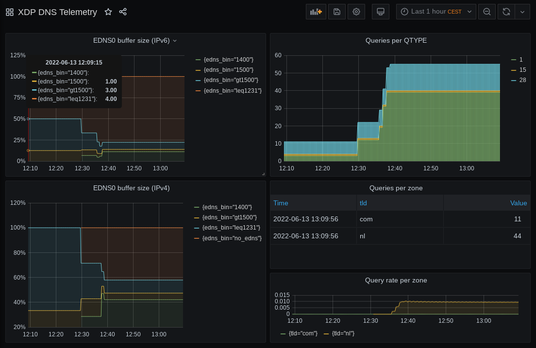
Finally, we turned the printed statistics into some eye candy. Even without any significant Grafana-fu (like yours truly) its easy to create a simple but useful dashboard like the example below (Figure 1). And there you have it: from incoming DNS queries to visualised telemetry.
Gathering DNS statistics for telemetry purposes using XDP is easy
In the end, we found gathering of DNS statistics for telemetry purposes as described to be relatively easy. And, most if not all of the benefits we enjoyed in previous XDP programs also apply here: A performant, drop-in solution, without the need to reconfigure or reboot an already running system. The code is available on GitHub.
Our lessons learned and final recommendations are:
- Picking the right map is key.
- Not try to do everything in BPF; find balance. Calculating rates from the answer counts is something Prometheus is designed to do anyway, so we did not bother. Doing some prep work by binning the response sizes is not too complicated and reduces processing further down the pipeline.
- Use maps as an interface. If you run something other than Prometheus, simply modify the userspace tool to print out the lines in a different format. Communication with kernel space via the map is no different.
In our next blog post, we’ll look at how we can implement a seemingly simple request we got from operators trying out our RRL program: Can we block queries based on the qname?
Acknowledgements
A big thank you to Ronald van der Pol and SURF for supporting us in doing these experiments, as well as APNIC for their editing and review of this article.
Contributors: Willem Toorop, Tom Carpay